Practical Statistics for Software Engineering - Distributions

Editor’s Note (Circa April 2023)

At the time of writing this I was pretty lax with terminology of “latency” vs “processing time”. There is a semantic difference between these words, but for the sake of this blog treat all usage of these words as “some measurement for time”.

Introduction

In the infinite list of topics that programmers are expected to know¹, I’m surprised statistics isn’t on this list.

I bring this up because in my (relatively short) career as a SWE, I’ve seen some questionable metrics and conclusions drawn from data. Initially I thought this was a “team” problem, after switching teams I thought it was a company one, but after changing companies I’m suspecting it might be more of an industry problem.

In the countless, required, intro statistics courses in my life - I never got the point until I actually used it on the job. So, I’m going to try to teach statistical lessons in a software context.

“Real World” Example - Response Latency Measurements

Determining response latency from logs seems straightforward, but I make the claim that this example is “realistic” because I’ve had similar experiences in this work.

Let’s say that we have all the logs in the past week relating to latency measurements (i.e no sampling). You’ve been asked some mission-critical questions like: “Do the latency numbers for X service match the < 90ms requirement?”

What’s the answer?

The Answer

The answer… depends. Questions like these can be tricky because finding the answer varies based on the “distribution” of the measurements, which you can think of as the relationship between a value (latency @ 20ms) and how frequently it occurs (number of logs corresponding to ~20ms latency).

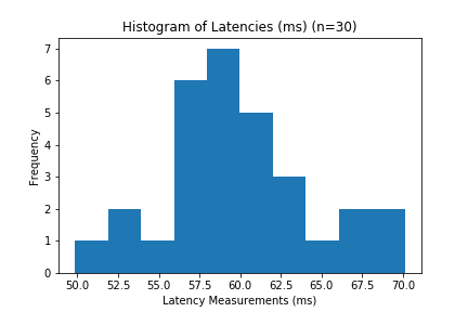
The first step is to visualize your data in a histogram. Using a histogram, we can get an idea of how frequently certain “buckets” of latencies appear to get an idea of our distribution. Answer,the previous questions involves digging through the data depending on what the distribution looks like.

Normal Distribution (Unlikely to happen)

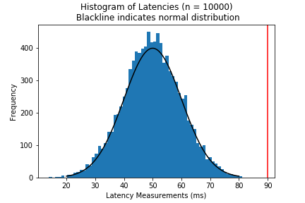
The “easiest” situation is if your data indicate that latencies falls along a normal distribution - a common distribution that fits a lot of other natural phenomena in life. Per the section heading, I’m highlighting that you won’t run into this distribution when working with latency, but could in other contexts.

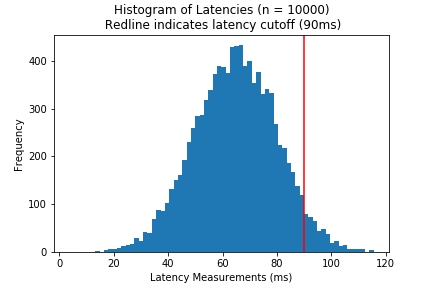
Actual data collected is likely to have outliers, so I added a few outliers around 270 ms that represents an abnormally slow response (maybe the server was incredibly slow that day, or the server has a undocumented behavior that causes hangs 1% of the time).

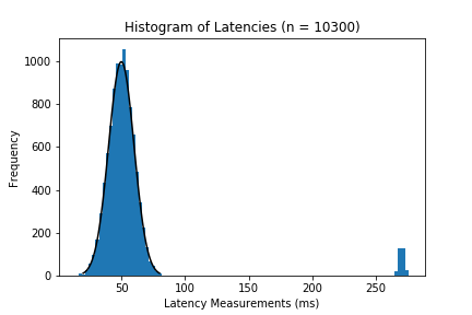
In this case, if we deem these latencies greater than 260ms, we’re going to just filter them out. However, outliers can be more subtle than that - don’t just ignore data points that make analysis difficult for you. Luckily, there are tools that can help identify outliers systematically (IQR rules, Z-scores, etc).

After filtering these out, the data will look something like the original figure (I’ve included the cutoff for clarity).

From the histogram, we can eyeball that the latencies are all under the 90ms goal - and that our service meets all latency requirements.

Normal Distribution Extended

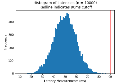
An alternative scenario may have a cutoff that intersects with the distribution like below:

If the data distribution seems normal, we can use the standard deviation to determine what’s “good enough”.

1. We can eyeball that the cutoff is a little more than 1 standard deviation (15ms) from the mean (65ms). Since we’re lazy we can use the 68-95-99.7 rule to estimate that the probability we get a latency greater or equal to 90ms is 16%

2. To be more precise, we can use the cumulative density function (cdf in most statistical libraries) to find a value.
   • The probability we have latencies greater than 1 STD is going to be less than 15.9%
   • Using python: 1 - scipy.stats.norm.cdf(1, loc=0, scale=1) = 15.9%
3. If we’re using scipy, we can calculate a tighter bound like so:
   • 1 - scipy.stats.norm.cdf(90, loc=65, scale=15) = 4.8%

This means that roughly < 5% of requests will not meet the cutoff. Whether this is acceptable or not is up to the person who made the cutoff.

Log-Normal

Latency measurements rarely follow a normal distribution, and are more likely to follow a distribution that looks like something like this:

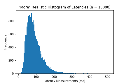
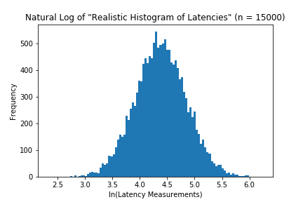
A distribution that fits this data is a log-normal distribution. The Log-normal is a distribution where its natural log is normally distributed (i.e if you were to take the natural log of latencies, the histogram would have a normal distribution).

If we’ve deemed the distribution is sufficiently normal, then we can use cdf function to answer the same questions as the normal distribution.

The next step is to find model parameters for our lognormal distribution. Most statistical libraries define lognormal distributions by their underlying normal distribution \~N(mean, std)

• Unfortunately, finding the model parameters of the underlying normal by taking the std and mean of the logged data (mu_norm, sigma_norm = np.mean(np.log(data)), np.std(np.log(data))) does not work.
• Instead we need to derive our model’s mean and std ($\mu_x, \sigma_x$) from our observed data ($\mu_y, \sigma_y$) using these formulas: ${\mu}_x = ln(\frac{\mu_y^2}{\sqrt{\sigma_y^2 + \mu_y^2}})$, ${\sigma}_x^2 = ln(\frac{\sigma_y^2 + \mu_y^2}{\mu_y^2})$ ²
  • For our example, we calculate a mu_x = 4.37, sig_x = 0.51.

Now we need to know the likelihood that our service will have response latencies greater than 110ms. The calculation is 1 - scipy.stats.lognorm.cdf(110, s=sig_x, scale=np.exp(mu_x)) which is a 25.7% (not very good).

Multimodal Distributions

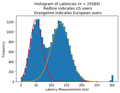
There are quirks in your data (such as multi-modality) that cannot be explained by skew, outliers, or different distributions. These quirks are better explained by quirks in your codebase, deployment process, user demographics, etc. Depending on the scale or software, there can be a rare flow in a request, difference with the request locations, or difference with the server’s location

For example, users in different parts of the world may have drastically different latencies. Below is an example of (hypothetical) latency measurements where the server is located in North America while its users might be located in the US and EU (with similar users across both).

Another example is that a new change to your codebase causes processing speed to be slower. Below is an example of (hypothetical) latency measurements where some server runs an older version of the code while a smaller number of servers run a newer, slower version of the code.

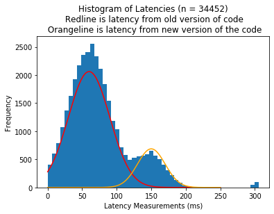
Both of these distributions are multimodal distributions - which is a distribution with multiple modes. Just note that this isn’t always the case.

Dealing with these situations involve separating out these groups into different sections (if you can) by filtering by a field, adding new data to your measurement process, or employing mixture models to try to differentiate these groups.

A Note: Erlang Distribution

I’m not an expert on this subject, but I’m going to mention Erlang Distributions (a subset of Gamma distributions) because I want the reader to be aware of alternatives.

There’s seems to be conversation on the best distribution to fit latency distributions. This NewRelic post indicates that an Erlang distribution is a better fit than Log-normal, but the 2001 paper “What Do You mean?-Revisiting Statistics for Web Response Time Measurements.” mentions that Erlang distribution don’t fit as well³. The helpfulness of this information is unclear, but could be helpful later!

Conclusion

This was a “starting off” discussion of distribution models to understand latency performance in software. As a reminder, these examples don’t represent the intricacies and limitations when working with real data - furthermore I jumped into using cumulative distribution functions without even talking about probability density functions (big theory gap here). I recommend doing some more readings/research (that’s not on the internet) or consulting with experts to learn more.

As a controversial stance, I’d note that that “rigorous statistics” should not always be the point of these exercises. Methodological correctness & rigor are ideal, but precision isn’t always necessary. Estimating is fine, especially when it’s a number managers don’t prioritize⁴! I would also note that there are nefarious reasons to lazy statistics, such as individuals intentionally misleading others about performance metrics.

Q & A

How can you determine if data follows a certain theoretical distribution?

There are several techniques, and a basic one I was taught is Q-Q plots. I always encourage research into more techniques or consulting an expert.

Is there a difference between working with sample latencies and the whole population of latencies?

Yes - there is so much of a difference between a sample and a population that I discourage applying techniques covered without further research.

How did you generate these histograms

I used the provided functions within np.random to generate normal and lognormal distributions to generate data, and matplotlib to generate the figures.

To generate multimodal distributions, I combined two different normal distributions like so:

import numpy as np

dist1 = np.random.normal(50, 20, 1000)
dist2 = np.random.normal(100, 10, 1000)
combined = np.concatenate([dist1, dist2])

Why is it scale=np.exp(mu_x) instead of mu_x?

I’m not sure, and this caused me a lot of confusion when I was learning about lognorm in scipy. Especially considering that parameter s (standard deviation) would be set to the standard deviation of the underlying normal dist, but scale is set to the mean of the lognormal distribution.

Footnotes